Table of Contents
1. Anomaly Detection
2. Phases of Matter and Anomaly Detection – A motivating example from quantum many-body physics
3. Quantum Autoencoder Model
4. Our Research
4.1. Application of the Quantum Autoencoder for Fraud Detection
4.2. Quantum Support Vector Machines – Separation and Reconstruction in the Hilbert Space
5. Challenges and Outlook
6. Further Reading
7. Bibliography
1. Anomaly Detection
In data analysis, anomaly detection refers to the often semi- or unsupervised task of identifying patterns, observations, or events that demonstrate significant deviations from the expected or normal behavior within a dataset. These outliers or novelties may represent rare events, errors, fraud, or other interesting phenomena that differ in some way from the majority of the data. Examples of anomalies are shown in Figure 1.
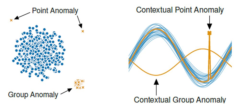
Figure 1: Different type of anomalies [1]
In the semisupervised case, the training data contains only samples which are assumed to be normal, whereas in the unsupervised case, the data has no labels at all. In addition, the datasets are usually highly unbalanced, i.e., there are far fewer anomalies than normal instances. These restrictions make semi- and unsupervised anomaly detection in general more challenging than supervised learning.
Anomaly detection has wide-ranging applications in fields such as finance, healthcare, industrial monitoring, as well as in cybersecurity and fraud detection, where the detection of unusual occurrences or behaviors can have significant implications for identifying potential security threats. Due to the increasing availability of vast amounts of data, traditional rule-based methods may struggle to effectively handle the scale and complexity of modern datasets. As a result, Machine Learning has become an important approach in anomaly detection, leveraging algorithms and models to automatically identify patterns and anomalies in large-scale datasets. These approaches are capable of processing and analyzing vast amounts of information to uncover hidden patterns and detect deviations from expected behavior. Furthermore, success has been shown in analyzing and identifying anomalies from massive datasets.
In principle ML approaches can be divided into at least four detection paradigms, which are based either on probability, classification, compressibility or the distance of points. Whether a point is an anomaly with respect to these paradigms, then depends on whether an anomaly is a
- comparatively rare event,
- differs from normal points in terms of its features,
- is more difficult to describe or compress than normal data,
- or is in some geometrical sense far away from normal data.
In this article we will present two approaches we have been investigating in the research group Quantum Security Technologies at Fraunhofer AISEC using a quantum computer for anomaly detection.
The first approach is inspired by the problem of phase recognition in quantum many-body physics, which shows some remarkable parallels to the field of anomaly detection, while the second approach can be visualized very well geometrically.
2. Phases of Matter and Anomaly Detection – A motivating example from quantum many-body physics
What are phases of matter? In our everyday life we mainly deal with three phases: solid, liquid and gaseous. Everybody has a basic intuition about how these phases are related to external parameters such as temperature, how transitions between phases occur and what the properties of the different phases, e.g., of water, are. However, when moving to more exotic materials such as superconductors, there is a whole zoo of exotic phases (superconducting, spin density wave, charge density wave, symmetry protected phases, et al.) which are not that straightforward to describe or identify without apriori knowledge (e.g., a so-called order parameter) of the system.
Nevertheless, from the perspective of Machine Learning, this is just an anomaly detection problem: If one phase is known it can be defined as the »normal phase« while other phases are different kinds of anomalies.
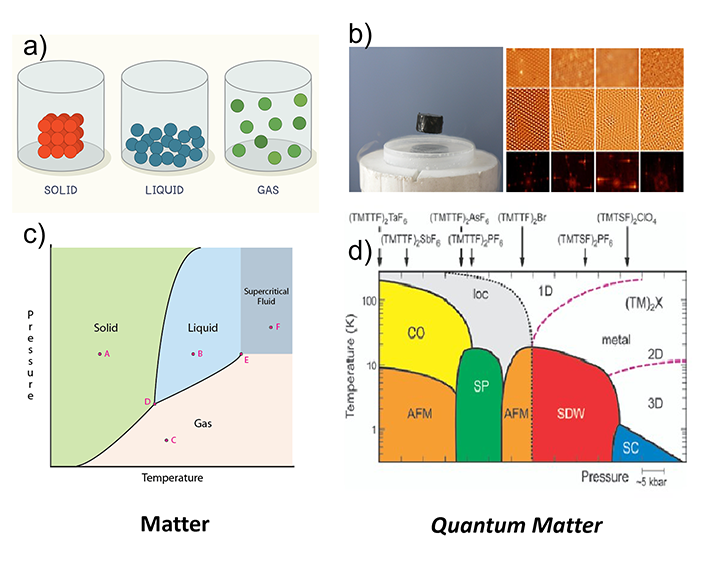
Figure 2: a) Phases of every day matter we all know. b) Superconductivity and charge density waves [Image credit: Stephan Rosenkranz]. c) Phase diagram of »normal matter«. d) Phase diagram of »quantum matter« (organic superconductors (TMTTF)2X – »Fabre Salts«) [2]
An important tool for studying many-body systems is the quantum phase diagram. It is a map of the different phases that a system can exist in, as a function of various parameters like the temperature, pressure, or magnetic field. Quantum phase diagrams can be used to identify the critical points at which a system transitions from one phase to another. Critical points are often associated with interesting and exotic physical phenomena, such as superconductivity and superfluidity. Since we usually want to know the phase of the ground state of our system, it is important to know what the ground state is. Here the quantum computer comes into play, as it can be used to find the ground state of our system with an algorithm called Variational Quantum Eigensolver (VQE). If apriori information about the quantum system is known one could now proceed and measure the so-called order parameter that can be used to distinguish two phases. If no information about the system is available (quantum) machine learning approaches, in particular anomaly detection, can be employed to »learn« the phases of the quantum system. One such approach is the so-called Autoencoder. How the VQE and a Quantum Autoencoder can be utilized to create a quantum phase diagram is described below.
3. Quantum Autoencoder Model
The Quantum Autoencoder (QAE) is a quantum algorithm that can be used to compress data or to perform classification tasks. The algorithm consists of two parts and the final measurement, as shown in Figure 4. The first part, the embedding layer, embeds the data samples into the circuit. This is followed by the variational layer consisting of parametrized gates whose parameters are optimized during training of the model. Finally, the measurement gives the output of the model, which can be a reconstruction loss, a label or any other metric that is useful for the classification task.
Now, let’s go back to the previous example of determining the phase diagram of quantum matter. Since our data is from the quantum realm and the operating principle of a quantum computer is based on quantum physical effects, these devices are ideally suited for creating the phase diagram of our system. For the embedding layer, the VQE comes into play, which achieves two goals: First, it can determine the ground state of the system, i.e., its lowest energy state. Second, it prepares quantum states in a way that we can apply our variational layer to them. Finally, the measurement assigns an anomaly score to the quantum state, whereby the higher the score, the higher the probability that the state is anomalous. Now, we define our ground state as the normal state and train our model with it. After the training has completed, we use the model to predict anomaly scores for many different quantum states. The resulting phase diagram can be seen in Figure 3. If the anomaly score is low, the state is in the phase we defined as »normal« and if the score is high, the state is in a different, non-normal, phase. Since the anomaly score increases abruptly as soon as the state is no longer in the »normal phase«, the phase boundaries are clearly visible. If the system has a second anomalous phase, the two anomalous phases can be identified by a difference in the anomaly score. This means, we can generate the whole quantum phase diagram after training our model with only one single quantum state!
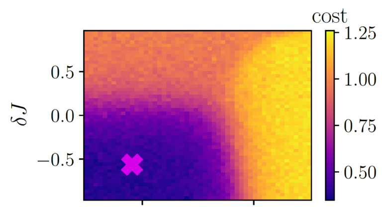
Figure 3: Quantum phase diagram determined by classification with a Variational Quantum Circuit. The single quantum state used for training the model is marked by the »x«. The color shows the cost or anomaly score, which can be understood as a measurement of how anomalous the phase is. [3]
Why does this work? We embed our state in a fixed number of qubits, let’s say five, as shown in Figure 4. After applying the variational circuit, we will measure only a subset of the qubits. In our example we will measure two of the five qubits. Our loss is the average number of 1s in the bit-string of measurement outcomes, so when we measure the states and both with probability 0.5, our loss will be 0.25. During training, we optimize the parameters of the variational circuit in such a way that the loss for the normal sample(s) is as low as possible. This means, the model is trained in the manner that the measured qubits are zero with high probability for the normal samples. Hence, the measured qubits do not contain information about the normal samples and the information about these samples is compressed from five to three qubits. For this reason, the measured qubits are called trash qubits. Now, if the model’s input is an anomalous sample, due to its different structure, it is usually not possible to compress the data into only three qubits and the trash qubits will be nonzero with high probability which results in an increased loss for these samples.
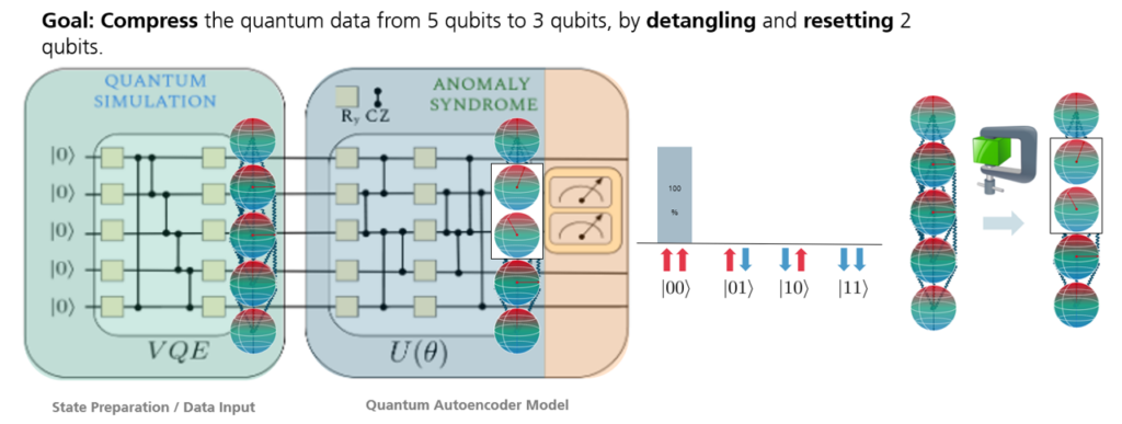
Figure 4: Architecture of the quantum autoencoder with embedding layer. The bar diagram shows the output probabilities of the two trash qubits. The spheres show the output states of a normal sample before and after training of the model. Each sphere represents one qubit, and the red line shows the state of the qubit. If the line points to the top (bottom), the qubit is in state \(\mid 0\rangle\) (\(\mid 1\rangle\)). Before training, the states of the trash qubits are in a superposition of \(\mid 0\rangle\) and \(\mid 1\rangle\) and the loss is large. After training, the trash qubits are in a state close to \(\mid 0\rangle\) and the loss is small.
4. Our Research
4.1. Application of the Quantum Autoencoder for Fraud Detection
We adapted the QAE for anomaly detection in financial transactions. Our approach is similar to the one described above with the difference that we deal with nonquantum data. The intuition behind this is, that if the QAE can be used to create a quantum phase diagram, why not use it to create a phase diagram for classical data, e.g., to find fraudulent financial transactions. Hence, instead of a quantum phase diagram, we want to obtain a »fraud phase diagram«, as sketched in Figure 5. (However, it must be noted that due to the complexity of real-world datasets and the necessary preprocessing such as dimensionality reduction, the »fraud phase diagram« won’t be as intuitive as depicted any more).
We trained the model with a few samples of a credit card fraud dataset and benchmarked the model on both normal and fraudulent transactions afterwards. We showed that the QAE can indeed distinguish between these two types of transactions. Moreover, we benchmarked the model also on other real-world datasets as well, like network intrusion, DNS over HTTPS traffic, or detecting malicious URLs.
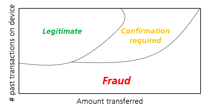
Figure 5: Sketch of a fraud phase diagram for financial transactions.
4.2. Quantum Support Vector Machines – Separation and Reconstruction in the Hilbert Space
A different approach developed by researchers at Fraunhofer AISEC is the Quantum Support Vector Regression (QSVR) for anomaly detection. This method is based on the Support Vector Machine, a classifier that uses a kernel to improve the separation of two different classes. The kernel maps the data from its initial space, the feature space, to the higher dimensional kernel space, as shown in Figure 6. In this example, the kernel space has an additional dimension which is the distance to the origin. In this three-dimensional kernel space, the data can be separated by a hyperplane which is not possible in the initial feature space.

Figure 6: The kernel enables linear separation of two classes in kernel space that is not possible in feature space.
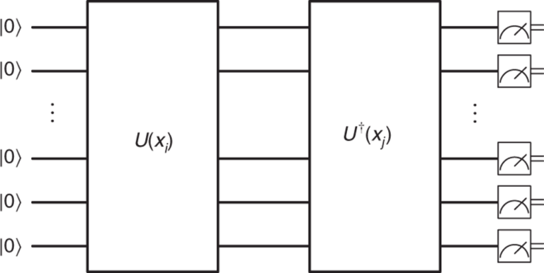
Figure 7: general architecture of a quantum kernel. [4]
The difference between a Support Vector Machine and Support Vector Regression is that the SVR uses the kernel to perform a constrained linear regression on it, as shown in Figure 8. We train our model so that it learns to predict one of the input features, and we use multiple SVRs to get a prediction of all input features. Our anomaly score, that classifies the samples as normal or anomalous, is then the reconstruction loss between the predicted features and the real input features. Our experiments showed that this approach works very well for many different datasets, including credit card fraud and other cybersecurity datasets.
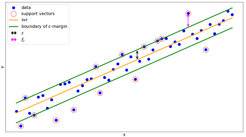
Figure 8: Regression task solved by the SVR. \(\in\) is a hyperparameter and \({\xi}\) defines by how much the sample is out of the \(\in\)- margin.
5. Challenges and Outlook
Although the results above are very interesting, they were obtained in simulations and not on real hardware, since currently available quantum computers are prone to errors and have low coherence times. These limitations of current hardware have not yet allowed researchers to show a practical quantum advantage, i.e., a problem that was solved on a real quantum computer but cannot be solved or only be solved exponentially slower on a classical computer. Even though quantum computers are theoretically superior to classical computers for some problems, it remains to be seen when and if a quantum advantage can be demonstrated in experiments. Our current research focuses on optimizing our QSVR model for real hardware and finally benchmarking it on a real quantum computer.
6. Further Reading
This blog post is based on our paper »Semisupervised Anomaly Detection using Support Vector Regression with Quantum Kernel« which was presented at IEEE Internal Conference on Quantum Computing and Engineering (QCE23).
Read the preprint here: https://arxiv.org/abs/2308.00583
7. Bibliography
[1] Ruff et al., »A Unifying Review of Deep and Shallow Anomaly Detection«
[2] Dressel et al., »Comprehensive Optical Investigations of Charge Order in Organic Chain Compounds (TMTTF)2X«
[3] Kottmann et al., »Variational quantum anomaly detection: Unsupervised mapping of phase diagrams on a physical quantum computer«
[4] Liu et al., »A rigorous and robust quantum speed-up in supervised machine learning«
Author

Kilian Tscharke
Kilian Tscharke has worked at Fraunhofer AISEC since 2022. As part of the Quantum Security Technologies (QST) group he specializes on Anomaly Detection using Quantum Machine Learning. Part of his work is embedded in the Munich Quantum Valley, an initiative for developing and operating quantum computers in Bavaria. Here, he focuses on Quantum Kernel methods like the Quantum Support Vector Machine that use a quantum computer for the calculation of the kernel.
Contact: kilian.tscharke@aisec.fraunhofer.de
